Asymptotic approximations

This example demonstrates the validity of the asymptotic approaches of approximating the thermodynamics of the freely-jointed chain (FJC) model in the modified canonical ensemble. For more information, see Buche and Rimsza, 2023.

To start, import and create an instance of the FJC model in the modified canonical ensemble:

import numpy as np
import matplotlib.pyplot as plt
from polymers import physics
fjc = physics.single_chain.fjc.thermodynamics.modified_canonical.FJC(8, 1, 1)

Strong potential

For sufficiently strong potentials, the modified canonical ensemble can be accurately approximated using the reference system (the isometric ensemble) and an asymptotic correction. For example, the nondimensional force \(\eta\) as a function of the nondimensional potential distance \(\gamma\) is approximated as

\[\eta(\gamma) \sim \eta_0(\gamma) - \frac{1}{N_b\varpi}\left[\eta_0(\gamma)\,\frac{\partial\eta_0(\gamma)}{\partial\gamma} - \frac{1}{2N_b}\frac{\partial^2\eta_0(\gamma)}{\partial\gamma^2}\right]\quad\text{for }\varpi\gg 1,\]

where \(\varpi\equiv\beta W\ell_b^2\) is the reduced nondimensional potential stiffness, \(N_b\) is the number of links, and the nondimensional force \(\eta_0\) for the freely-jointed chain model in the isometric ensemble as a function of the nondimensional end-to-end length per link \(\gamma\) is given by

\[\eta_0(\gamma) = \frac{1}{N_b\gamma} + \left(\frac{1}{2} - \frac{1}{N_b}\right)\frac{\sum_{s=0}^{s_\mathrm{max}}(-1)^s\binom{N_b}{s}\left(\frac{1-\gamma}{2} - \frac{s}{N_b}\right)^{N_b - 3}}{\sum_{s=0}^{s_\mathrm{max}}(-1)^s\binom{N_b}{s}\left(\frac{1-\gamma}{2} - \frac{s}{N_b}\right)^{N_b - 2}},\]

where \(s_\mathrm{max}\leq (1-\gamma/2)N_b \leq s_\mathrm{max}+1\). In contrast, the exact relation for \(\eta(\gamma)\) is obtained by numerically evaluating

\[\eta(\gamma) = -\frac{1}{N_b}\frac{\partial}{\partial\gamma}\,\ln\left[\iiint Q_0(\boldsymbol{\gamma}') \, e^{-\tfrac{\varpi}{2} N_b^2\left(\boldsymbol{\gamma} - \boldsymbol{\gamma}'\right)^2} d^3\boldsymbol{\gamma}'\right],\]

where \(Q_0\) is the partition function in the isometric ensemble. This exact relation is plotted below along with the asymptotic relation while varying \(\varpi\), the nondimensional potential stiffness. As \(\varpi\) increases, the asymptotic approach appears to do increasingly well, but always eventually fails as \(\gamma\) becomes large. This is because the asymptotic approach in this case is completely invalid for larger values of \(\gamma\) (approaching 1), where the massive associated entropic force would cause the end of the chain to leave the bottom of the potential well, even though it may be quite strong. It is therefore apparent that \(\varpi\gg\eta\) in addition to \(\varpi\gg 1\) is a requirement for the asymptotic relation to succeed in accurately approximating the full system.

gamma = np.linspace(1e-3, 99e-2, 256)
for varpi in [1e0, 1e1, 1e2]:
    eta = fjc.nondimensional_force(gamma, varpi)
    line = plt.plot(gamma, eta, label=r'$\varpi=$' + str(varpi))
    eta_asymptotic = \
        fjc.asymptotic.strong_potential.nondimensional_force(gamma, varpi)
    plt.plot(gamma, eta_asymptotic, ':', color=line[0].get_color())
plt.legend()
plt.xlim([0, 1])
plt.ylim([0, 12])
plt.xlabel(r'$\gamma$')
plt.ylabel(r'$\eta$')
plt.show()

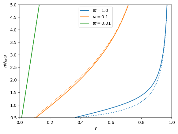
Weak potential

For sufficiently distant potentials, the modified canonical ensemble can be accurately approximated using the reference system (the isotensional ensemble) and an asymptotic correction. The potential is considered sufficiently distant when the length of center of the potential well to the end of the chain experiencing it is much larger than the expected end-to-end length of the chain. This disparity in length is only typically possible considering weak potentials. For example, if \(\eta/N_b\varpi\) is the nondimensional potential distance, the nondimensional end-to-end length per link \(\gamma\) as a function of the effective nondimensional potential force \(\eta\) is approximated as

\[\gamma(\eta) \sim \gamma_0(\eta)\left[1 - N_b\varpi\,\frac{\partial\gamma_0(\eta)}{\partial\eta}\right]\quad\text{for }\varpi\ll 1,\]

where \(\gamma_0(\eta)=\mathcal{L}(\eta)\) for the freely-jointed chain model in the isotensional ensemble, and where \(\mathcal{L}(x)=\coth(x)-1/x\) is of course the Langevin function. In contrast, the exact relation for \(\gamma(\eta)\) is obtained by numerically evaluating

\[\gamma(\eta) = \frac{1}{N_b}\frac{\partial}{\partial\eta}\,\ln\left[\iiint Q_0(\boldsymbol{\gamma}') \, e^{N_b\boldsymbol{\eta}\cdot\boldsymbol{\gamma}'} e^{-\tfrac{\varpi}{2} N_b^2\left(\boldsymbol{\gamma}'\right)^2} d^3\boldsymbol{\gamma}'\right].\]

This exact relation is plotted below along with the asymptotic relation while varying \(\varpi\), the nondimensional potential stiffness. As \(\varpi\) decreases and/or the nondimensional force \(\eta\) increases (the nondimensional potential distance \(\eta/N_b\varpi\) increases), the asymptotic approach appears to do increasingly well. Notably, the asymptoic approach appears to succeed for sufficiently distance potentials for any value of \(\varpi\). This is because the freely-jointed chain model has inextensible links, so even a stiff potential that is distant (\(\eta/N_b\varpi\gg 1\)) will not stretch the chain past \(\gamma=1\). For chain models which have extensible links, the link stiffness will compete with the potential stiffness, such that the potential would need to be weak (\(\varpi\ll 1\)) in addition to distant (\(\eta/N_b\varpi\gg 1\)) in order for the asymptotic approach to become accurate.

gamma_in = np.linspace(5e-1, 5, 256)
for varpi in [1e0, 1e-1, 1e-2]:
    gamma = fjc.nondimensional_end_to_end_length_per_link(gamma_in, varpi)
    line = plt.plot(gamma, gamma_in, label=r'$\varpi=$' + str(varpi))
    gamma_asymptotic = \
        fjc.asymptotic.weak_potential.nondimensional_end_to_end_length_per_link(gamma_in, varpi)
    plt.plot(gamma_asymptotic, gamma_in, ':', color=line[0].get_color())
plt.legend()
plt.xlim([0, 1])
plt.ylim([0.5, 5])
plt.xlabel(r'$\gamma$')
plt.ylabel(r'$\eta/N_b\varpi$')
plt.show()